定义

1. Precision plot: percentages of frames whose estimated locations lie in a given threshold distance to ground-truth centers.
   追踪算法估计的目标位置（bounding box）的中心点与人工标注（ground-truth）的目标的中心点，这两者的距离小于给定阈值的视频帧的百分比。不同的阈值，得到的百分比不一样，因此可以获得一条曲线。一般阈值设定为20个像素点。
   该评估方法的缺点：无法反映目标物体大小与尺度的变化。
   比如一个视频有101帧，追踪算法预测的bounding box中心点与ground-truth中心点距离小于20像素有60帧，其余40帧两者距离均大于20个像素，则当阈值为20像素时，精度为0.6。

2. Success Plot: Let rt denote the area of tracked bounding box and ra denote the ground truth. An Overlap Score (OS) can be defined by S = |rt∩ra| |rt∪ra| where ∩ and ∩ are the intersection and union of two regions, and | · | counts the number of pixels in the corresponding area. Afterwards, a frame whose OS is larger than a threshold is termed as a successful frame, and the ratios of successful frames at the thresholds ranged from 0 to 1 are plotted in success plots.
   首先定义重合率得分（overlap score，OS），追踪算法得到的bounding box（记为a），与ground-truth给的box（记为b），重合率定义为：OS = |a∩b|/|a∪b|，|·|表示区域的像素数目。当某一帧的OS大于设定的阈值时，则该帧被视为成功的（Success），总的成功的帧占所有帧的百分比即为成功率（Success rate）。OS的取值范围为0~1，因此可以绘制出一条曲线。一般阈值设定为0.5。

各种追踪算法中precision plots和Success plots如下：

上述定义摘抄自：https://blog.csdn.net/hjl240/article/details/52453030

实现

输入文件

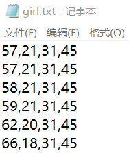
1. 自己跑某个算法得到的结果为每一帧要跟踪的物体坐标，如下图所示：
   

2. 给出的标准答案：
   

3. 显然我们发现描述一个四边形有多种形式，在第一象限下：
   a. 矩形框左下坐标+宽和高
   b. 矩形框中心点坐标+宽和高
   c. 矩形框左下坐标+右上坐标
   d. 四边形的四个点的坐标

一点点解释

1. get_axis_aligned_bbox() 函数的作用是把上文3中c 和d 坐标，转成a 的形式。参考博客：https://blog.csdn.net/l1127071087/article/details/93794003
2. 下面最后四行代码显然是我们使用的关键。readData() 函数读入文件地址，数据的间隔符和是否需要进行坐标转换。如果文件内坐标是上文3中a的形式，就输入False。showPrecision 和 showSuccess 函数读入各个算法跑出来的数据，标准数据，算法名和曲线颜色。

代码

import numpy as np
from matplotlib import pyplot as plt

# 规范化矩形描述方式
# 传入四点或两点坐标返回，一点的坐标加宽高


def get_axis_aligned_bbox(region):
    region = np.asarray(region)
    nv = len(region)
    if nv == 8:
        cx = np.mean(region[0::2])
        cy = np.mean(region[1::2])
        x1 = min(region[0::2])
        x2 = max(region[0::2])
        y1 = min(region[1::2])
        y2 = max(region[1::2])
        A1 = np.linalg.norm(region[0:2] - region[2:4]) * \
            np.linalg.norm(region[2:4] - region[4:6])
        A2 = (x2 - x1) * (y2 - y1)
        s = np.sqrt(A1 / A2)
        w = s * (x2 - x1) + 1
        h = s * (y2 - y1) + 1
        return (cx - w / 2, cy - h / 2, w, h)
    else:
        return (region[0], region[1], region[2] - region[0], region[3] - region[1])

# print(get_axis_aligned_bbox([28.788,57.572,97.714,57.116,98.27,141.12,29.344,141.58]))

# 传入两个矩形的左下角和右上角的坐标，得出相交面积，与面积


def computeArea(rect1, rect2):
    #  让rect 1 靠左
    if rect1[0] > rect2[0]:
        return computeArea(rect2, rect1)
    # 没有重叠
    if rect1[1] >= rect2[3] or rect1[3] <= rect2[1] or rect1[2] <= rect2[0]:
        return 0, rect1[2] * rect1[3] + rect2[2] * rect2[3]
    x1 = max(rect1[0], rect2[0])
    y1 = max(rect1[1], rect2[1])
    x2 = min(rect1[2], rect2[2])
    y2 = min(rect1[3], rect2[3])

    rect1w = rect1[2] - rect1[0]
    rect1h = rect1[3] - rect1[1]
    rect2w = rect2[2] - rect2[0]
    rect2h = rect2[3] - rect2[1]
    return abs(x1 - x2) * abs(y1 - y2), rect1w * rect1h + rect2w * rect2h - abs(x1 - x2) * abs(y1 - y2)

#print(computeArea([-3,0,3,4], [0,-1,9,2]))

# 从文件读入坐标


def readData(path, separator, need):
    reader = open(path, "r", encoding='utf-8')
    ans = []
    lines = reader.readlines()
    for i in range(len(lines)):
        t = lines[i].split(separator)
        t = [float(i) for i in t]
        if need:
            ans.append(get_axis_aligned_bbox(t))
        else:
            ans.append(t)
    return ans


def getCenter(region):
    return (region[0] + region[2] / 2, region[1] + region[3] / 2)


def computePrecision(myData, trueData, x):
    # 获取中心差
    cen_gap = []
    for i in range(len(myData)):
        x1 = myData[i][0]
        y1 = myData[i][1]
        x2 = trueData[i][0]
        y2 = trueData[i][1]
        cen_gap.append(np.sqrt((x2-x1)**2+(y2-y1)**2))
    # 计算百分比
    precision = []
    for i in range(len(x)):
        gap = x[i]
        count = 0
        for j in range(len(cen_gap)):
            if cen_gap[j] < gap:
                count += 1
        precision.append(count/len(cen_gap))

    return precision


def computeSuccess(myData, trueData, x):
    frames = len(trueData)
    # 获取重合率得分
    overlapScore = []
    for i in range(frames):
        one = [myData[i][0], myData[i][1], myData[i][0] +
               myData[i][2], myData[i][1] + myData[i][3]]
        two = [trueData[i][0], trueData[i][1], trueData[i][0] +
               trueData[i][2], trueData[i][1] + trueData[i][3]]
        a, b = computeArea(one, two)
        overlapScore.append(a / b)

    # 计算百分比
    precision = []
    for i in range(len(x)):
        gap = x[i]
        count = 0
        for j in range(frames):
            if overlapScore[j] > gap:
                count += 1
        precision.append(count/frames)

    return precision


def showPrecision(myData, trueData, algorithm, colors):
    # 生成阈值，在[start, stop]范围内计算，返回num个(默认为50)均匀间隔的样本
    xPrecision = np.linspace(0, 10, 20)
    yPrecision = []
    for i in myData:
        # 分别存放所有点的横坐标和纵坐标，一一对应
        yPrecision.append(computePrecision(i, trueData, xPrecision))

    # 创建图并命名
    plt.figure('Precision plot in different algorithms')
    ax = plt.gca()
    # 设置x轴、y轴名称
    ax.set_xlabel('Location error threshold')
    ax.set_ylabel('Precision')

    for i in range(len(myData)):
        # 画连线图，以x_list中的值为横坐标，以y_list中的值为纵坐标
        # 参数c指定连线的颜色，linewidth指定连线宽度，alpha指定连线的透明度
        ax.plot(xPrecision, yPrecision[i], color=colors[i], linewidth=1,
                alpha=0.6, label=algorithm[i] + "[%.3f]" % yPrecision[i][-1])

    # 设置图例的最好位置
    plt.legend(loc="best")
    plt.show()


def showSuccess(myData, trueData, algorithm, colors):
    # 生成阈值，在[start, stop]范围内计算，返回num个(默认为50)均匀间隔的样本
    xSuccess = np.linspace(0, 1, 20)
    ySuccess = []
    for i in myData:
        # 分别存放所有点的横坐标和纵坐标，一一对应
        ySuccess.append(computeSuccess(i, trueData, xSuccess))
    # 创建图并命名
    plt.figure('Success plot in different algorithms')
    ax = plt.gca()
    # 设置x轴、y轴名称
    ax.set_xlabel('Overlap threshold')
    ax.set_ylabel('Success')

    for i in range(len(myData)):
        # 画连线图，以x_list中的值为横坐标，以y_list中的值为纵坐标
        # 参数c指定连线的颜色，linewidth指定连线宽度，alpha指定连线的透明度
        ax.plot(xSuccess, ySuccess[i], color=colors[i], linewidth=1,
                alpha=0.6, label=algorithm[i] + "[%.3f]" % ySuccess[i][0])

    # 设置图例的最好位置
    plt.legend(loc="best")
    plt.show()


girlData = readData(r"D:\Desktop\STRUCK-master\build\Release\girl.txt", ",", False)
girlDataTrue = readData(
    r"D:\Desktop\STRUCK-master\build\sequences\Girl\groundtruth_rect.txt", "\t", False)

showPrecision([girlData], girlDataTrue, ["Struck"], ["r"])
showSuccess([girlData], girlDataTrue, ["Struck"],["r"])

运行结果